Methods applicable to the study of active faults
The concept of active fault is a subject of many studies all over the world. The history of this concept in the world and especially in Russia was reviewed by V.G. Trifonov (Trifonov, 1983; Trifonov, 1985; Trifonov, 2000). In the USSR and Russia we should acknowledge great contribution in the methods and regional studies of active faulting of: K.E. Abdrakhmatov, S.G. Arzhannikov, A.V. Arzhannikova, V.S. Burtman, A.V. Chipizubov., V.S. Imaev, L.P. Imaeva, T.P. Ivanova, R.M. Lobatskaya, N.V. Lukina, O.V. Lunina, V.I. Makarov, E.A. Rogozhin, S.F. Skobelev, O.P. Smekalin, A.L. Strom, S.I. Sherman, A.V. Vakov.Extremely detailed systematic descriptions of methodological and practical aspects of the study of active faults presented in two editions of "Paleoseismology" edited by James P. McCalpin (Paleoseismology, 1996, 2009), “Geology of Earthquakes” by Robert S. Yeats, Kerry E. Sieh, and Clarence R. Allen. (Yeats et al., 1997), and "The Mechanics of Earthquakes and Faulting” by Christopher H. Scholz (Scholz, 2002).
What is an active fault?
First of all, it is necessary to define the term "active fault", as its meaning strongly affects identification and mapping of active faults. Active fault identification is the most crucial and complex aspect in active fault studies, and it required a deep insight into the nature of fault tectonics.Two properties of active faults are most common among the varying definitions of the term:
1), a possibility (or expectation) of slip in the near geological future and 2), time (or age) of the last slip (e.g. Slemmons and DePolo, 1986). Almost the same concept was stated by N.A. Florensov as early as 1963 (Florensov, 1963, p. 381), “...The most objective indicator of the possibility of earthquakes in the future is, undoubtedly, the evidence that they occurred in this area in the past”.
A possibility (or expectation) is the basis of the term "active fault". An active fault is a fault with possible future slip. The expectation of future movement is what make geologists consider the fault as an active, whereas all other parameters (i.e. sense, slip rate, etc.) are properties of any fault disregarding its age, and, therefore, does not indicate its activity. Possibility of the future slip makes it crucial to account active faults before the construction of any important object, and vice versa, inactive faults have no chance to directly affect the construction. Figures 1, 2 and 3 below are photos of earthquake ruptures created by the most recent but likely not the last movements on active faults that deformed the Earth’s surface.
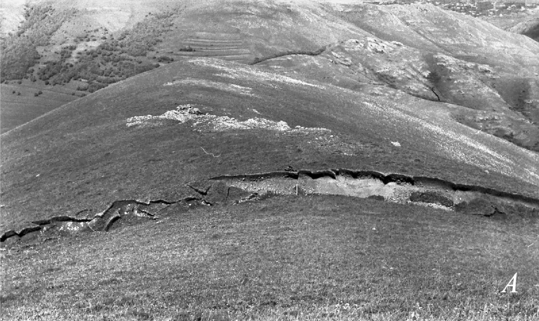
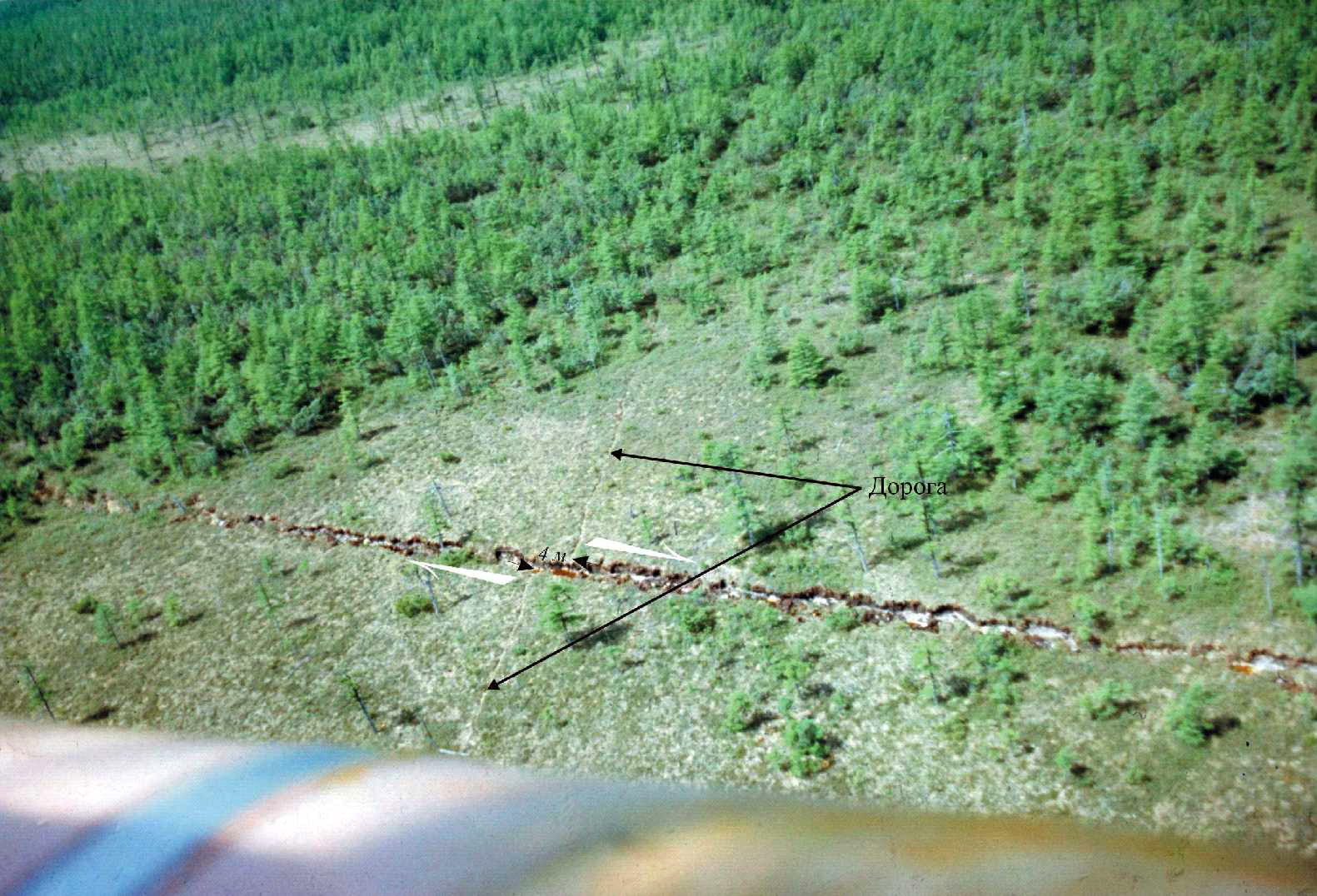
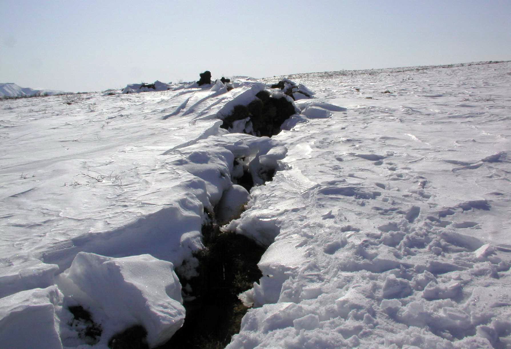
Fig. 1. Surface rupture of the Spitak Earthquake (1988, Ms = 6.8). Photo by A.I. Kozhurin.
Fig. 2. Surface rupture of the Neftegorsk Earthquake (1995, Ms = 7.1). Photo by A.I. Kozhurin.
Fig. 3. Olutorskoye (or 2006 Kamchatka) Earthquake (2006, Mw = 7.6). Photo by T.K. Pinegina.
Age of the last slip is a clue for the possibility of the future slip when considered together with recurrence interval of slip events.
General assumptions of the maximum interval are following: According to K. Allen (Allen, 1975), its duration is ~ 10 ka, i.e. approximately Holocene time. V.G. Trifonov proposed (1983, 1985) to expand it up to 100-130 ka for orogenic belts, and up to 700 ka for stable geologic provinces, whereas A.A. Nikonov (1995) considered ca. 400 ka as a maximum interval of slip events.
Most of faults moves episodically by slip events and stay quiescent for hundreds and thousands of years, even if distant (e.g. 10-15 km) points on its sides accumulate displacement gradually. That displacement cause stress accumulation at the fault plane, which discharge through elastic rebound (Reid, 1910). after exceeding the limit of rock tensile strength, and result in an earthquake. However, geodetic surveys show that a few faults slip almost constantly without seismicity, those are termed creeping faults.
Let’s assume that we study a fault with motions occurred every ~2 kyr, but the most recent one occurred 10 ka. The quiescence has been lasting for several average recurrence intervals (Fig. 4, A) and it’s unlikely that the fault is still active. Another case: the most recent slip 0.5 ka have been identified on a fault with the same recurrence interval of ~2 kyr. As the recurrence interval has not passed since the slip, next slip is likely to occur in the future, and the fault should be considered active.
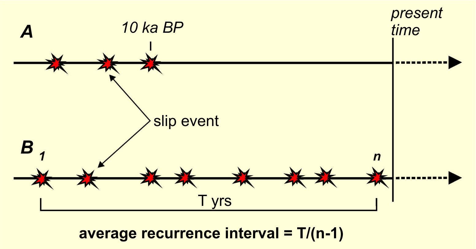 Fig. 4. A hypothetical model of movements on the fault. A, inactive fault. B, active fault (redrawn from Kozhurin et al., 2008).
This model helps understand generally assumed maximum intervals mentioned above. These threshold values of 10 – 700 ka imply a possible maximum recurrence interval according to the global statistics and provide best possible estimate if no recurrence interval is known for some specific fault from field or instrumental data.
Our hypothetical recurrence interval of 2 ka is realistic; both shorter and longer intervals are known. For example, Umehara fault (Japan) ruptured ca. every 14-15 kyr (Okada et al., 1992). Within the Kamchatka Peninsula, identified recurrence intervals vary from 9 ka (Kozhurin et al., 2008) to 2 ka (Zelenin et al., 2020). Considering possibility of missing the most recent event on a poorly studied fault, we may increase expected interval up to 20 ka, even double or triple this value, increasing our confidence, and interpret motions within that range as a sign of an active fault. In the same manner V.G. Trifonov reasoned maximum interval for faults of orogenic belts (Trifonov, 1983, 1985, 2000).
This approach was summarized by A.I. Kozhurin et al., (2008): a possibility of a future slip is what defines an active fault, an expectation of future slip is based on evidences of movement on the fault during the last tens of thousands of years.
Identification and mapping of active faults
Slip that occurred some tens of thousands of years ago affects topography, even rather young Late Pleistocene - Holocene landforms. Displacement of landforms is versatile and practical indicator of active faulting.The exact landscape expression of an active fault relies on the type of displaced landforms and fault sense. The most common expression is a fault scarp, with height varying along the strike (Fig. 5 and 6 are examples from the Kamchatka Peninsula).
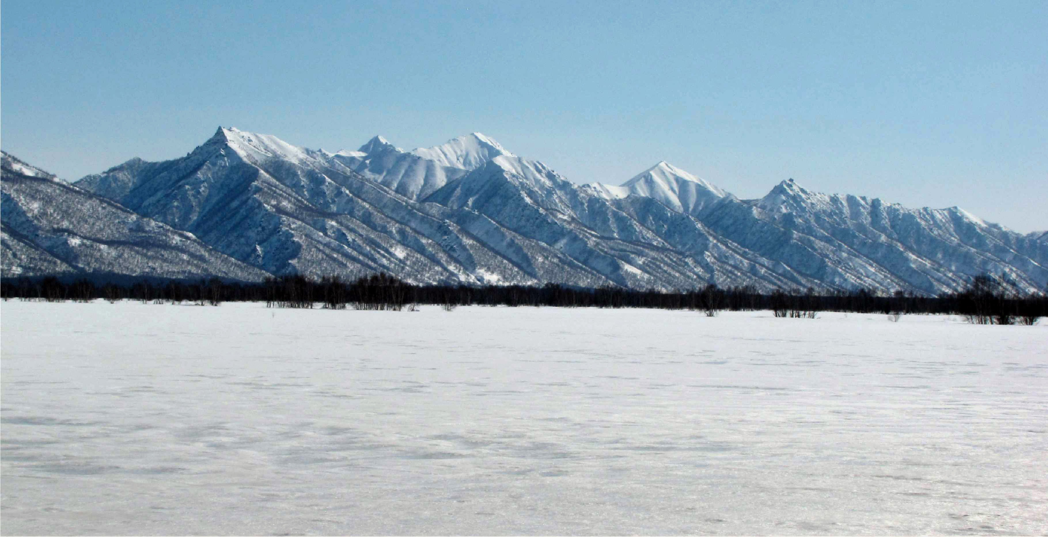 Fig. 5. Faceted spurs along the normal fault scarp dividing the Central Kamchatka Depression and the Eastern Ranges. The altitude of the Ganalsky Ridge above the depression floor is about 1 km at the photo. View to SE. (photo by A.I. Kozhurin).
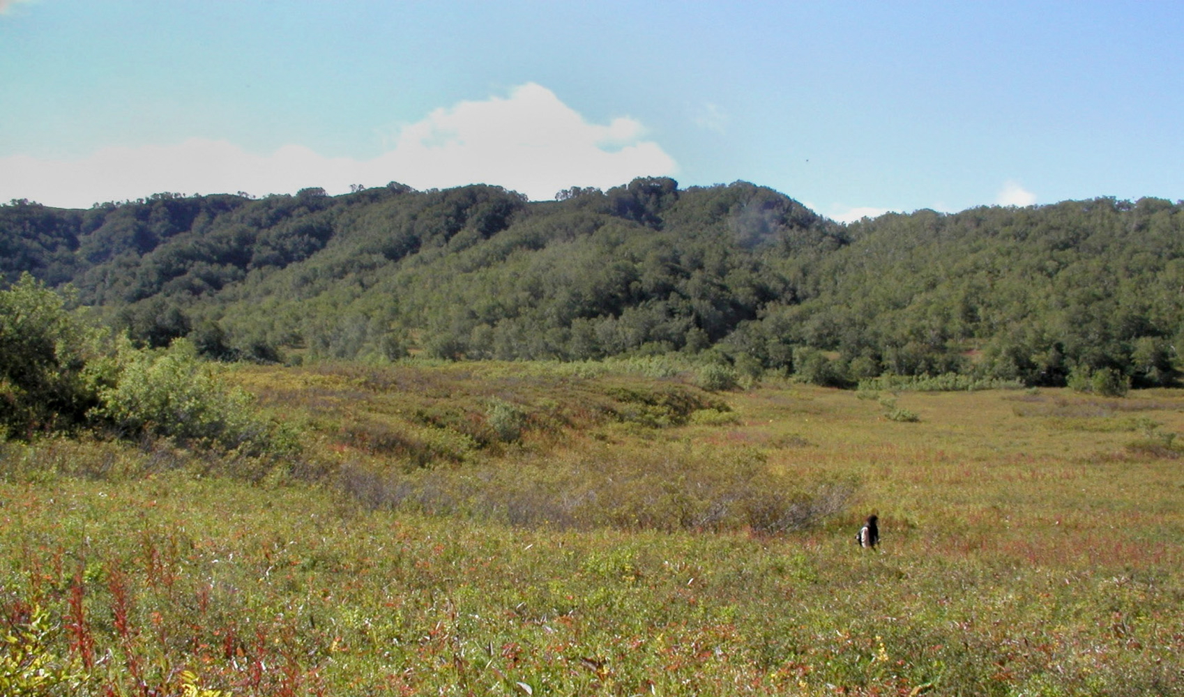 Fig. 6. Fault scarp deforming the surface of the upper postglacial terrace of Bol'shaya Khapitsa River (the Kumroch Ridge). View to the south (photo by A.I. Kozhurin). See Fig. 12. for the paleoseismological interpretation of a trench across the fault.
Besides dip-slip faults, scarps emerge along strike-slip faults as well: horizontal shift of fault walls on a rough terrain will match landscapes of different height. Note that the apparent vertical offset at a strike-slip fault scarp should not be considered as the vertical throw without correction for heave.
Since active faults deforms landscape, they can be detected on remote sensing data, from aerial photographs to satellite imagery. Figures 7 and 9 illustrate how active faults appear in imagery.
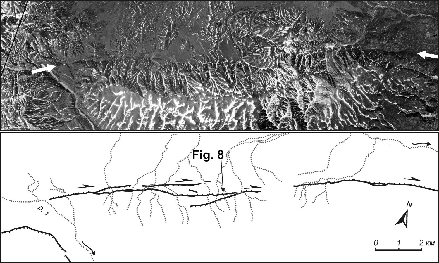 Fig. 7. Right-lateral strike-slip fault in SE Kamchatsky peninsula, Kamchatka (by Kozhurin et al., 2014). Top, an aerial photograph with white arrows located along the fault line. Bottom, a sketch map of drainage pattern and fault scarps, arrow indicates location of photo on Fig. 8.
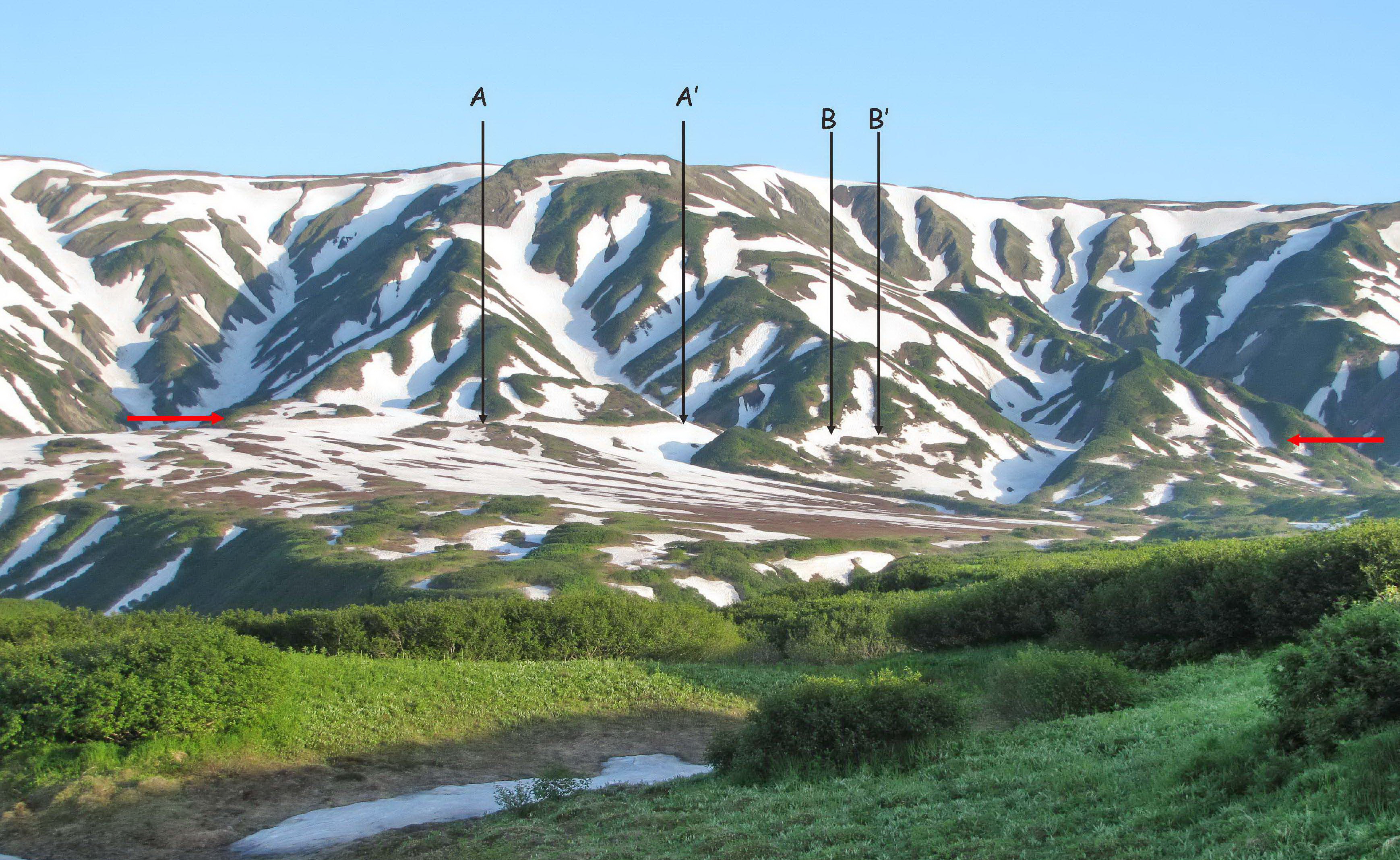 Fig. 8. A photo of right-lateral strike-slip fault in SE Kamchatsky peninsula, Kamchatka. View to the south. Red arrows indicate fault trace. AA' and BB' – landforms offset by about 150 m (AA’) and 35 m (BB’) (Kozhurin et al. 2014). Photo by A.I. Kozhurin
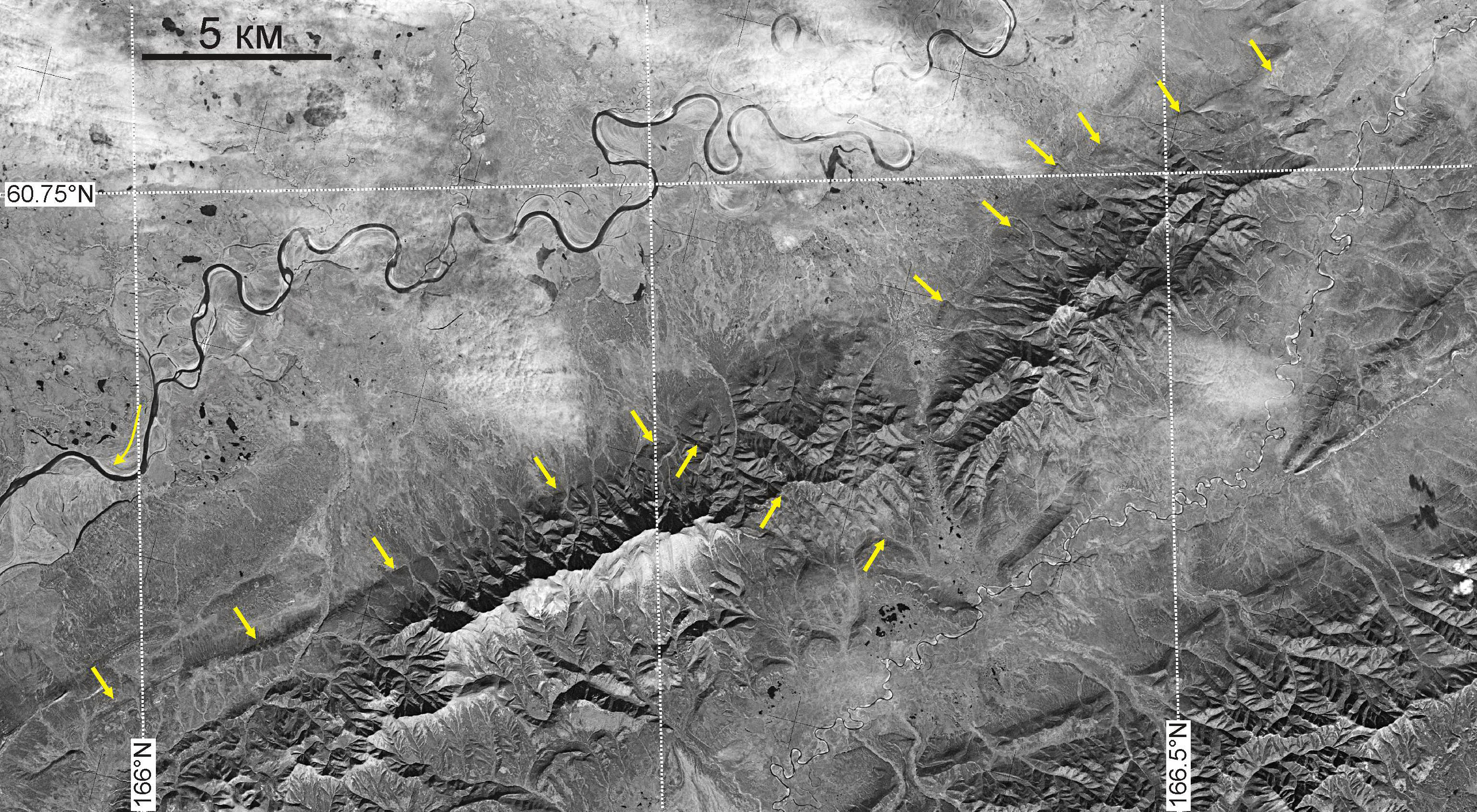 Fig. 9. Right-lateral strike-slip active fault in Koryak Highland on KH-9 Hexagon space image. Yellow arrows indicate fault trace (by Pinegina, Kozhurin, 2010). The most recent slip on this fault occurred in AD 2006 (Olutorskoe or 2006 Kamchatka Earthquake, Mw = 7.6).
Despite faulting produce generally uniform set of landforms, accurate interpretation of every individual case requires specific study. There are several general rules of such interpretation (for details see Trifonov et al., 1993; Kozhurin et al., 2008; Trifonov, Kozhurin, 2010):
1. Linear landform that resembles fault trace should be studied for their non-tectonic (e.g. fluvial, glacial, coastal) origin.
2. As fault slip accumulates over time, older landforms should be offset more than younger ones. A classic illustration of this phenomenon from the Athera Fault in Japan (Fig. 10) was provided by A. Sugimura and T. Matsuda (1965). Fig. 8 is one more example of an increasing displacement of a larger (and older) valley.
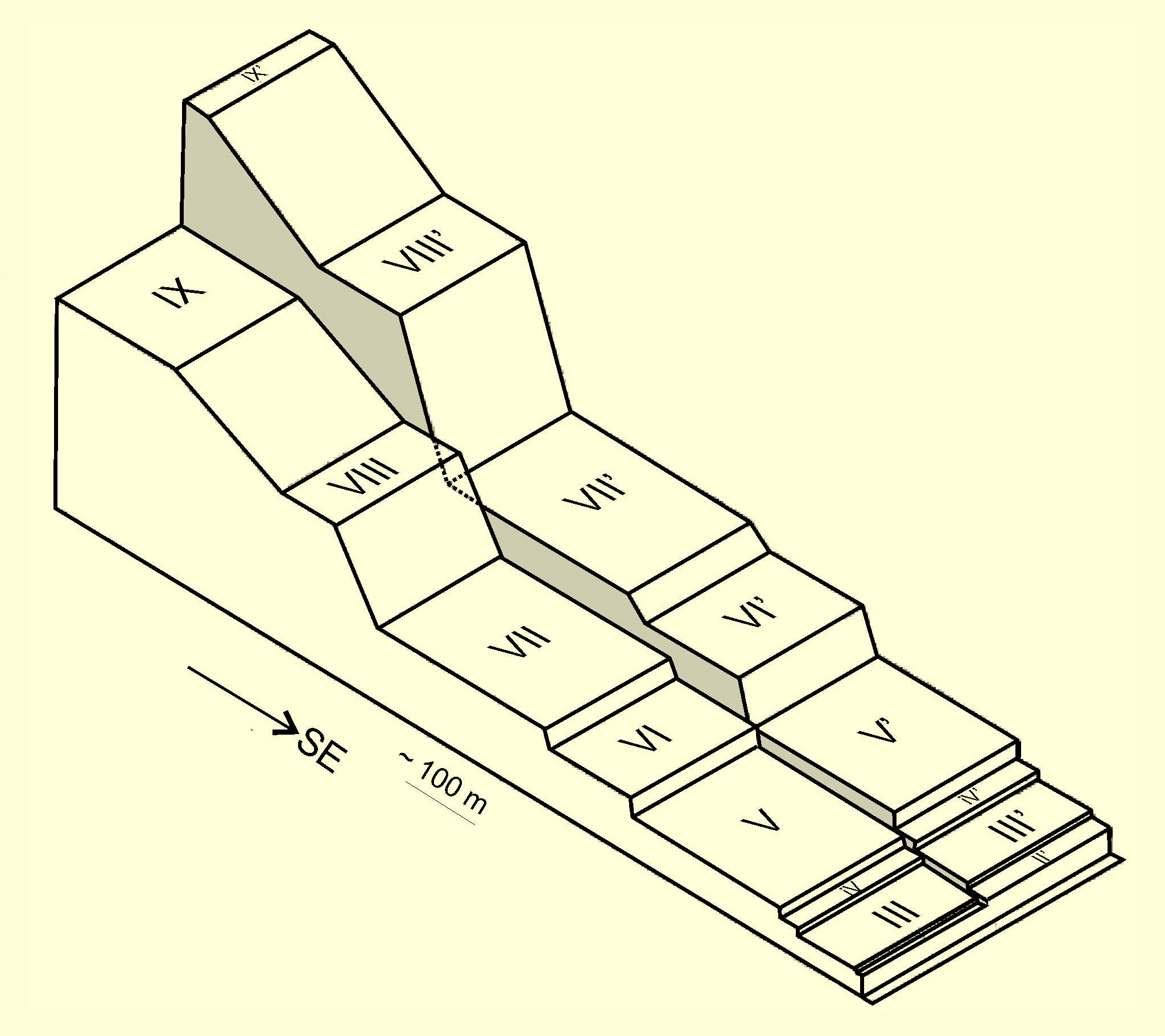 Fig. 10. Left-lateral deformation of Kiso river terrace sequence at the Atera Fault, central Honshu, Japan (redrawn from Sugimura and Matsuda, 1965). Roman numerals identify terraces from young to old. The offset increases from 17 m at the terrace II to 140±35 m at the terrace IX.
3. The supposed fault must fit general pattern of regional neotectonics; active faults comprise a subset of neotectonic faults.
This list helps distinguish active faults and lineaments, which is commonly confused. The latter do not displace surface in a uniform style increasing on older surfaces, but usually form tectonically impossible regular systems (orthogonal and diagonal), which invariably densify with an increase in the scale of analyzed data.
Methods of studies of active faults
After identification of an active fault on remote sensing data, the field study of the fault starts from geomorphological survey. Natural outcrops of a fault plane are often insufficient for the study, so they may be supplemented my man-made excavations across the fault scarp, particularly important when fault deforms recent sediments.The kinematic analysis of fault slip is a versatile tool providing data for main fault characteristics such as attitude, sense, estimation of average slip rate.
Detailed study of slip timing and rupture dimensions require specific approach, paleoseismology, based on interpretation of sediments and landforms disturbed by prehistoric earthquakes. Both geomorphological survey and man-made excavation address the very top of the fault plane, which is affected by surface processes partially induced by fault movements. Interpretation of disturbed sediments vary from simple cases of only one movement, to complex and ambiguous, when deformations superimpose each other. In the latter case, more trenches across the same plane may clarify the faulting history. Paleoseismological studies in Kamchatka, NW Pacific revealed the full range of cases, with deformation highlighted by contrast tephra layers (Fig. 11, 12).
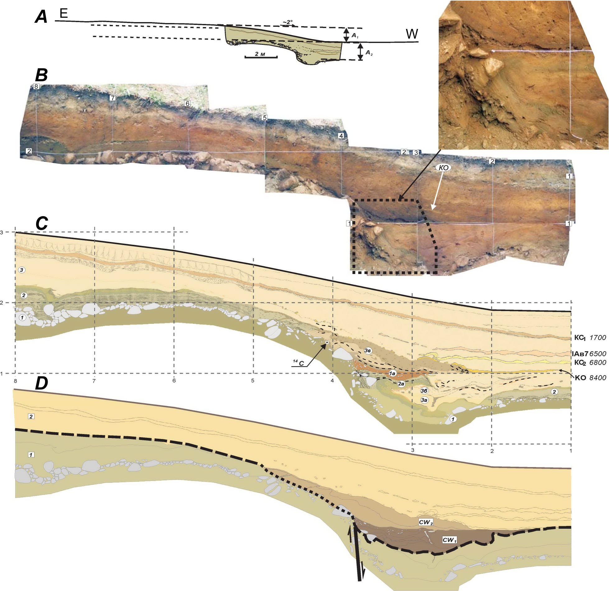 Fig.11. A simple structure of a disturbed section (one movement) at the southern wall of the Poperechnaya trench (redrawn from Kozhurin et al., 2008).
A. Topographic profile across the fault scarp at the trench site: A1, the offset of the Earth's surface, A2, the offset of the top of boulder alluvium.
B. Photomosaic of the trench wall with 1-m grid
C. Sketch of the section. Tephra horizons with their calendar age are labeled at the right, sedimentary units marked by numbers in circles.
D. Paleoseismological interpretation of the section: figures in squares - sediments accumulated before movement (1) and after movement (2); CW1 and CW2 - lower coarse and upper fine components of the colluvial wedge; dashed line shows the event horizon, approximate in the footwall; dotted line shows eroded surface of fault scarp.
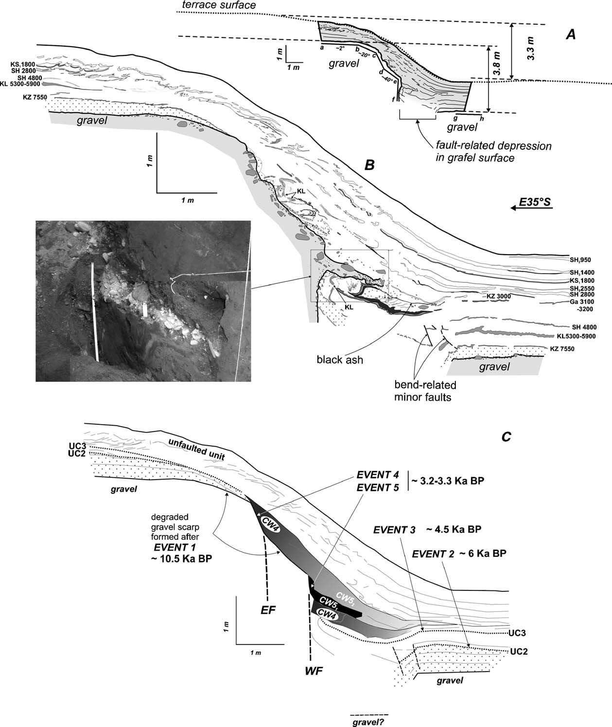 Fig.12. A section disturbed by several slips at the Bol'shaya Khapitsa trench (redrawn from Kozhurin et al., 2006).
A. Topographic profile across the fault scarp at the trench site, measured are offsets of the Earth's surface and of the top of gravel alluvium. The latter labeled abcdef and gf, where ab and gf are segments of the original surface in gravel, bc, de are eroded fault scarps and cd, ef are steeper segments above two fault planes.
B. Sketch of the section. Tephra horizons with their calendar age are labeled at the right.
C. Paleoseismological interpretation of the section: EF, East fault plane; WF, West fault plane, UC, unconformities; CW, colluvial wedge. Numbers in the labels for unconformities and colluvial wedges correspond to the number of the seismic event from older to younger: 10.5 ka, 6 ka, 4.5 ka, two events in 1.3-1.2 ka.
Slip events on the active fault affect landscape either, so they can be revealed, for example, on the histogram of the horizontal offset of landforms along the fault. A constant creep will constantly offset every landform crossing the fault, so that older landforms will be offset more than younger ones, and larger offsets will gradually decrease in number. If slip accumulates over time by seismic events, the offsets will comprise of some single-event displacements, close in magnitude (say, n meters), and the histogram will have peaks at n, 2n, 3n, … meters (Fig. 13).
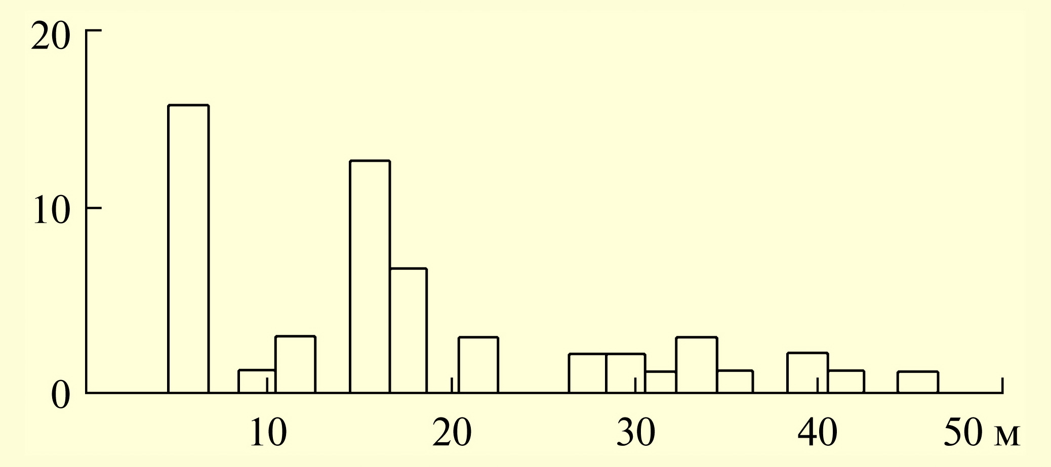 Fig. 13. Amount of measurements vs. horizontal offset diagram for late Holocene left-lateral displacements of small landforms on 15-km-long segment of Khangai fault along northern slope of Dagan-Del Ridge, Northern Mongolia (redrawn from Trifonov, 1983).
The peak at 5-6 m corresponds to the most recent Bolnai earthquake 23.07.1905, M > 8. Following peaks at 11±1; 16.5±1.5; 22±0.5; 28.5±1.5; 33±1; 40±1; 45±1 m corresponds to the multiple of Bolnai earthquake slip.
The method should be supplemented by the dating of events. For the strike-slip Khangai Fault, this problem was solved by 14C dating of pull-apart basins and sag ponds. Lacustrine and peat filling in coseismic depressions yielded dates for eight earthquakes during the last 4.5 ka with recurrence interval of ~600 years (Trifonov, 1983).
Conclusion
The study of active faulting has two outcomes:1. Active faults are sources of earthquakes, so active faulting studies should support any project of seismic hazard assessment and mitigation. That is the main practical use of identification and mapping of active faults. Fault length and single-event displacement are proxies for the future earthquake magnitude.
2. Faults’ pattern and kinematics directly reflect the geodynamic setting of the deformed portion of the crust.
Studies of active faults consider late Quaternary tectonics, recent tens to hundreds of millennia. It is a rather brief period of natural history, so that tectonic evolution is left off the scope in most studies of active faults. Instead, a pattern of active faults is a “snapshot” of the late Quaternary tectonic settings providing uniform basis for large-scale studies linking geodynamic studies of Earth’s current state and classical geological methods.